Most realistic quantum field theories are far to complex to allow for an analytic solution. Therefore, from the earliest days, people have developed approximation schemes, wherein a small parameter is identified, and then an expansion in this parameter is performed. In many quantum field theories, the coupling parameter can be viewed as effectively being very small. The corresponding expansion (around a non-interacting model) is called “perturbation theory”. It is still in general a highly non-trivial task to compute the various orders in this expansion. One complicating factor is that, if the expansion is performed naively, one typically gets infinite results, thus requireing some sort of “renormalization”. The principles and algorithms underlying renormalization in Minkowski spacetime were identified in the 60s-70s in papers by Bogoliubov, Parasiuk, Hepp, and Zimmermann, with important practical improvements such as dimensional regularisation (introduced by `t Hooft and Veltmann) or the BRST-method (due to Becci-Rouet-Stora-Tyutin) added subsequently. Later complementary approaches were also developed, such as the Epstein-Glaser-method, or the renormalization group flow equation method of Wilson-Wegner-Polchinski.
It is not so clear from the outset what the basic principles underlying renormalization should be in curved space. One guiding principle in flat space is that renormalization should be local and respect the spacetime symmetry (Poincare-transformations). In most approaches, “locality” is manifestly preserved by restricting to local counterterms, and Poincare-invariance in practice serves to reduce the “renormalization ambiguities” to a finite number of constants (in “renormalizable theories”). While the concept of locality is evident also on a curved spacetime (one can also insist on local counterterms), it is not so clear what should replace the condition of Poincare invariance. An obvious idea would be to replace the notion of “special covariance”, i.e. invariance under Poincare transformations, by “general covariance”. However, it is not easy to see how to impose this condition in practice, since diffeomorphisms are not symmetries of a spacetime, but rather relate one spacetime to another. One is therefore led to the idea to investigate the relationship between QFT’s on different spacetimes.
The situation one has in mind is that one has one space-time, say $N$, which is is embedded in a larger space-time, $M$. If the embedding is such that there are no new null geodesics relating points in $N$ inside the bigger spacetime $M$, then one would expect that the quantum field theories on $M$ and $N$ should be related in a simple way by some sort of restriction. However, one has to think precisely what exactly one means by this, because there is no natural correspondence between states on different space times. For example, $N$ would normally have a boundary, so the specification of a state should somehow reflect a choice of boundary conditions on $N$, etc. Thus, it is best to formulate the relationship between quantum field theories on $M$ and $N$ not via states, but via the algebras of observables. For a free Klein Gordon field, these algebras are given by the relations described above, and we naturally have (denoting the algebras by $\mathcal{A}$) $\mathcal{A}(N) \subset \mathcal{A}(M)$.
In practice, perturbation series for the interacting quantum fields of a theory (such as $\phi^4$-theory, or Yang-Mills theory, etc.) are given in terms of so-called “Wick-products” and “time-ordered products” in the underlying free field theory. The first problem is that these are not already contained in the algebra $\mathcal{A}(M)$, so one has to pass to a bigger algebra $\mathcal{W}(M)$. A time ordered product is a map $T_n$ that associates with each collection of (classical) “composite fields” $\mathcal{O}_i$ an operator valued distribution $T_n(\otimes_{i=1}^n {\mathcal O}_i(x_i))$, where by “operator valued” one means that the output is a member of $\mathcal{W}$. A basic problem that comes up when trying to define these objects is to control their singularities. These typically occur when two or more spacetime points $x_i \in M$ are lightlike related, or coincident. To deal with the non-coincident configurations, one makes use of a mathematical tool called “microlocal analysis”. Microlocal analysis is basically a version of Fourier analysis on manifolds, except that the Fourier transform is performed only locally near a given configuration of points in $M$. Thus, one naturally deals not just with a set of momenta $k_i$ as in flat space, but with a collection of pairs $(x_i, k_i)$ where $k_i$ is in the cotangent space at $x_i$. UV-singularities correspond to collections $(x_i, k_i)$ near which the local Fourier transform does not decay under a rescaling $k_i \to \xi k_i$ with positive $\xi$. Such directions are collected in the wave-front-set, which is, for any distribution in $n$ variables $x_i \in M$, a subset of $T^* M^n \setminus \{ 0 \}$.
In the recursive construction of the time-ordered products $T_n$, one needs to control precisely this wave front set, since it characterizes the UV-singularities. In particular, the configurations of $x_i$’s which are lightlike related or coincident matter. One finds a geometrical description of the wave front set $WF$ of the expectation value of a time-ordered product in a suitably regular state $\omega$, denoted $\omega(T_n(\otimes_{i=1}^n {\mathcal O}_i(x_i)))$, in terms of embedded Feynman graphs, see the picture:
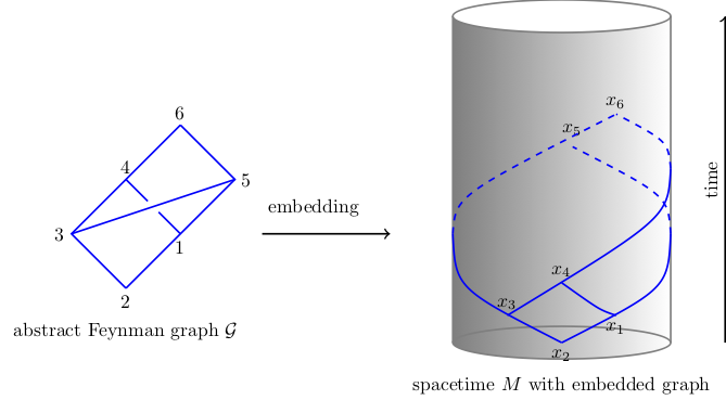
Shown here is the wave-front set of the time-ordered products and its relationship with embedded Feynman graphs $\mathscr{G}$ in $M$. The valence of the nodes of the graphs reflect the polynomial orders in $\phi$ of the $\mathcal{O}_i$’s. Through each line $e$ flows a `momentum’ $p_e$ indicated by an arrow, which is a parallel transported, cotangent null vector. At each vertex $x_i$ the corresponding vector $k_i \in T^*_{x_i} M$ in the wave front set is characterized by the `momentum conservation rule’ $k_i = \sum_{\rm in} p_e – \sum_{\rm out} p_e$ counting the momenta associated with the incoming vs. outgoing edges $e$ with opposite sign. Once one has the time-ordered products, one can, under certain circumstances, define the scattering matrix. For example, for interaction $L = \lambda \phi^4$, this would be given by
$$S = \sum_{n \ge 0} \frac{\lambda^n}{n!} \int_{M^n} T_n(\otimes^n_{i=1} \phi^4(x_i)) \ .$$
This expression is only formal, because, although the UV-problem is solved, there are new problems: The multiple spacetime integral over all of $M^n$ will usually not converge, and the infinite sum (over $n$) will not converge. The first problem reflects the fact that an $S$ matrix will usually simply not exist in curved spacetimes, i.e that it has an incurable IR divergence. This divergence is physical, and one should not even try to `cure it’ by some means. The second problem is that a perturbation series does not capture non-perturbative effects, i.e. quantities of interest in interacting QFT’s are usually not analytic functions in the coupling parameter ($\lambda$ in our example). While it is not known to us how to treat the second problem, there is a way to resolve the first problem. The idea is, again, to focus on the interacting fields of the theory. It turns out that these can be defined on any spacetime $M$, and it also turns out that on any spacetime $M$, there is a wide class of physical states. The interacting fields are given by infinite series involving $T_n$, so knowing these, one can, in principle calculate correlation functions of interacting fields in curved space-time. These are the objects to which the physical interpretation of a given state is tied.
Some references are:
- R. Brunetti and K. Fredenhagen: “Microlocal analysis and interacting quantum field theories: Renormalization on physical backgrounds,” Commun. Math. Phys. 208 (2000)
- S. Hollands: “Renormalized Yang-Mills theories in curved spacetimes”, Rev. Math. Phys. 20 (2008)
- S. Hollands and R. M. Wald: “Quantum field theory in curved spacetimes”, (a review with many references to original papers)